Finding Trends With Approximate Embedding Clustering

Clustering vectors by similarity is a powerful method to identify trends and categories of a dataset, frequently used in analytics (like identifying shopping trends) and in various AI use cases (like RAG and contextual tagging).

Many known algorithms exist to cluster data such as K-Means and Hierarchical Clustering, but based on implementation can be slow, memory-inefficient, and often rely on some data-prep stage that is not always available (such as dimensionality reduction, initial centroid selection, or a known value for k).

ClickHouse wrote a detailed post on accelerating K-means calculations at scale, but that method still suffers from all the data-prep requirements previously mentioned.

These algorithms aim at "converged" calculations: They iterate until they can't anymore. Not every use case for clustering needs to fully converge, often approximate solutions work great.

But they don't seem to exist, or at least are not well discussed or documented.

Why Approximations?

Many functions in ClickHouse (and other analytics tools) such as uniq and quantile are approximate aggregations to optimize for speed and memory usage, while you have to explicitly specify a -Exact variant of the function to get an exact result (which is slower and more resource intensive).

Why don't we have the same for vector clustering?

Well it turns out we do, and it's been flying under the radar as an initialization step for K-Means.

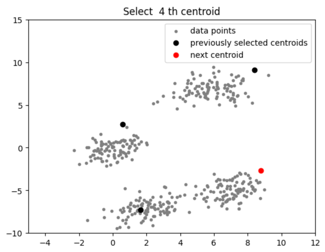
Approximate Clustering With K-Means++

The K-Means algorithm requires some initial centroids (the center of a cluster) to refine. The more accurate the placement, the quicker it can converge on accurate centroids. This post does a great job at explaining how it works.

K-Means++ is an initial centroid selection algorithm that is used to optimize the accuracy and speed of convergence for K-Means clustering.

Briefly, K-Means++ works by first selecting a random vector to serve as the first centroid, then looking for the furthest vector from each of the current centroids and selecting the minimum value as the next centroid, and so on until you have k number of centroids. You can find Python implementations here and here.

It does a pretty decent job at approximating cluster centroids:

The colab notebook can be found here.

Looking at that chart, it's pretty clear that we can use this as an accurate enough approximation to be useful.

Sure, there will be some vectors on the edges of the clusters that will likely fall into the wrong category, but since they're already close to the edges of an optimal centroid, that accuracy can be considered and tolerated.

Why Approximate Clustering?

At Tangia we set out to build a TTS (text to speech) copy-paste feature for our Better TTS product so that viewers could quickly find funny and trending TTS metas.

There were a few key requirements for this functionality:

1. The ranking algorithm should be able to identify trends (clusters) from TTS messages without any pre-existing knowledge of categories
2. Able to discover the number of relevant categories that exist in the dataset (find a decent k, not necessarily an optimal one)
3. Since TTS messages are often similar but not identical, the algo needs to be able to identify similar messages by context (embeddings)
4. A short TTL on rows so that old trends fade out, and maintained trends stay
5. Able to categorize newly added TTS messages to an existing trend (cluster) in real-time
6. Need to be able to discover new TTS trends quickly (rebuild clusters)

ClickHouse implementation of K-Means from their post was close to what we wanted, but it relied on a few things we didn't have or need like a known value of k, full convergence (e.g. iterating until centroids aren't moving any more), and reduced dimensionality (can't reduce dimensions when you're frequently inserting new records to the dataset at scale).

With K-Means++, we can get a decently accurate group of clusters, find k in the process (we'll discuss this a bit later), maintain the embeddings default dimensionality, and run rankings at query time within tens of milliseconds.

It has a simple polynomial sum runtime:

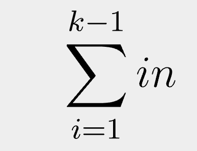
Where k is the number of clusters, i is the current iteration, and n is the number of vectors in the dataset.

This means with a k=6, it will be n + 2n + 3n + 4n + 5n to calculate the centroids. Not the fastest thing in the world, but way better than Hierarchical Clustering (HC), which is a "fully converging" method for finding clusters with an unknown value for k. HC is far more complex and a mega PITA to implement in ClickHouse SQL.

Dynamic K-Means++ with ClickHouse

To implement approximate clustering we need to set up a few tables and materialized views in ClickHouse.

I won't go over the SQL data piping since it's a bit hard to follow if you're not intimately familiar with ClickHouse, but the flow looks like this:

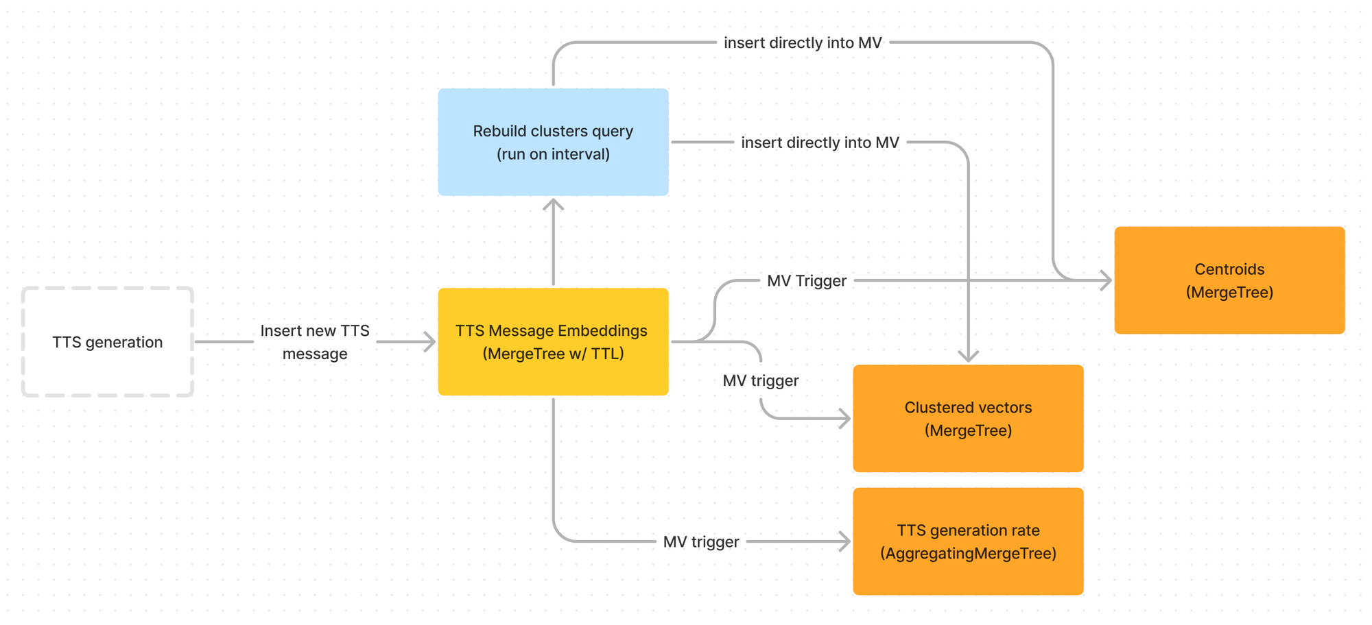
A notable distinction between this method and ClickHouse's implementation in their post is that we also store pre-computed cluster membership. This materialized view allows us to instantly order rows by (cluster, cluster_density, distance_from_centroid), giving us tens of millisecond access to find the current top-n records.

Finding k (Number of Clusters)

K-Means++ still requires some known value for k to decide when to exit.

While there are a few common methods for finding a good k value (such as the "elbow method"), with K-Means++ we can actually discover an appropriate value for k along the way.

Since every iteration of K-Means++ selects a new centroid, we can simply keep iterating until we hit some low-threshold of when to stop: For example when a single cluster makes up less than 15% of the number of points in the set.

This adds additional complexity to the runtime since we now need to iterate over the whole set again to assign points to the current centroids, but it's still quite fast.

Because the value of k is discovered dynamically, I'm calling this process "Dynamic K-Means++". "DKMPP" might be a hard acronym to catch on though...

We can also add some outlier resistance during centroid iteration by selecting the farthest point that's within some high percentile, like the 95th percentile (can be adjusted as required). This greatly reduces the chances that the next centroid is not ruined by an extreme outlier (although an unlucky first random centroid could do that).

-- (2) Find the furthest point from all centroids
select argMax(vector, max_dist), max(max_dist)
from (
  -- (1) Get the max distance to each centroid for all points
  select vector
    , arrayMax([
      L2Distance(vector, $centroid1)
      , L2Distance(vector, $centroid2)
      , ... -- each centroid
    ] as max_dist
  from points
)
-- keep under 95th percentile to protect against outliers
where max_dist < quantile(0.95)(max_dist)

The resulting vector is the next centroid. We can keep running this, including all newly selected centroids, until the following query returns a centroid that breaks our lower threshold:

-- (2) Find the ratio of centroid assignment
select
  count()/(select count() from vectors) as vec_ratio
  , centroid
from (
  -- (1) Find the closest centroid for each vector
  select (
    arraySort(
      c -> (c.2)
      , arrayMap(
        x -> (x.1, L2Distance(x.2, vector))
        , [[1, $centroid1], [2, $centroid2], ...] -- to currnet k
      )
    )[1]
  ).1 as centroid
  from vectors
)
group by centroid
having vec_ratio <= 0.15

If any centroid returns a vec_ratio below our threshold, we exit using current_k - 1 centroids.

Poor First Centroid Selection Resilience

While we found a great method for resisting outliers when finding subsequent centroids, there's still a chance that the first randomly selected centroid could be a massive outlier, and thus quickly trip our exit condition. While this probability varies greatly with the data, it's likely non-zero.

You could either choose to live with this probability, and we likely could get away with it at Tangia. After all, we do rebuild the clusters on a tight interval, so the lifetime of a bad calculation would be relatively short lived.

However, I decided this was easily avoidable with a simple trick:

1) Select N random first points to serve as potential first centroids

A clever way to randomly select row(s) is to randomly sort the points table by adding a sort_id Int64 Default rand64() column in your ordering key, generating a random 64-bit integer at insert time. Then you can select a random row extremely quickly like:

-- Get 5 random first centroid candidates
select *
from points
where sort_id >= rand64()
limit 5

This will always select a single granule, and does not slow down (notably) with more data.

2) Calculate the next centroid for each of the first points

Using the same query from earlier (with the outlier threshold) on each of our candidate first points.

3) Select the candidate with the closest subsequent centroid

The first centroid candidate with the closest second centroid is the least likely to be an outlier.

If they are all the same, then there is either no outlier, or the outlier is not far out enough to make a significant difference.

Increasing Approximation Accuracy

What if you need to be slightly more accurate than DKMPP?

You may recall that K-Means++ is an initialization step for K-Means, meaning (not a pun) that we can run K-Means to converge our cluster centroids closer to their optimal values.

There's no need to converage fully either, we can simply run a few iterations if we'd like just a bit more accuracy. After all, the earlier iterations have much more of an effect than the final iterations. I'll defer to ClickHouse's post on how to implement K-Means efficiently.

Recalculation Interval

When new TTS messages come in, they are immediately categorized into a cluster based on the closest centroid. This allows us to instantly add new TTS messages and rank them. This is important, because we get a lot of TTS messages.

Since categories can change, we fully-recalculate them every few minutes. A ground-up recalculation serves 2 purposes:

1. It identifies new clusters (TTS trends) that might emerge (including a change in k)
2. It allows us to TTL rows so that old trends get removed, while maintaining popular trends

Because there are periods of higher and lower activity during the day, we can dynamically adjust the rebuild interval to account for the rate at which TTS messages are created. That's a simple materialized view from our existing data to calculate the rate, with queries returning in tens of milliseconds.

This calculation is done largely with ClickHouse for performance. If you notice in the data flow diagram above, we use MergeTree for the materialized view targets instead of a ReplacingMergeTree. This is because we drop all existing rows from materialized view target tables before recalculating to keep the data set very small, and all previous centroids and cluster memberships are irrelevant after a rebuild.

Ranking Clusters

There are 2 tiers of ranking that need to take place:

1. The trend in TTS (which cluster)
2. The messages within the trend (which points inside the cluster)

Conveniently, they are both quite simple steps.

To find a TTS trend, we simply look at the most dense cluster (not the largest). Density of a cluster generally indicates that messages are very similar to each other, suggesting a stronger trend. This is somewhat sensitive to the inaccuracy of the approximate calculation, but since it's rotated so often it evens out over time.

This gets stored in a materialized view so that the density gets updated as new TTS message vectors are inserted.

Ranking messages within the trend is easy: Middle out.

The centroid of the cluster is the most similar to the trend, so we can simply sort from the euclidean distance to the centroid. This is also sensitive to the approximation accuracy, but since we only need to give a general idea, the accuracy is sufficient.

In reality, to add some variation, we take a top-n list by distance from the centroid and randomize it to give some variation in results.

Conclusion

I'm certainly no expert in vector clustering. In fact, I've only known about it for the last 60 hours or so.

It's pretty simple to wrap your head around, and quick to find how powerful it can be.

With approximate clustering, we can get a good idea how data can be categorized with very little prior info. It can give us a good direction to chase for more detailed analysis, show us quickly evolving trends, and works especially well on extremely large data sets.

It might not be appropriate for deciding stock trades or fraud analysis, but it sure works well for suggesting funny TTS ideas to live stream viewers.

Discuss on HackerNews: https://news.ycombinator.com/item?id=40189395